A contact arc in a circuit breaker is an extremely complex electro-thermo-hydro-dynamic process and that we never fully mathematically describe the detailed physics of an arc.  Our goal, here, is to develop an approximate arc model such that we can treat an arc as a circuit element, and analyze electric circuits containing arcs.

During normal circuit breaker operation, the arc, when present, is in a continual state of change.  It is dynamically lengthened by parting contacts and by electromagnetic forces which push it away from its original trajectory.  It is dynamically heated by its current.  It is dynamically cooled by its environment and, perhaps, by other auxiliary means (forced gas flow, cool containment walls, etc.).  And, dependent on the net rate of energy absorption (heating minus cooling), it dynamically grows in cross-sectional area.

As the arc changes physically and thermally, it also changes electrically.  A change in the electrical characteristics of the arc, in turn, changes the amount of through current that the external electrical circuit can supply.  Therefore, an engineering description (which is all that we seek) of a circuit breaker arc must include a dynamic description of the breaker-electrical network interaction.  Now, we will discuss the components of an electrical arc:  Cathodes, Anodes and Plasma Columns.

The two arc electrodes are referred to as the cathode and the anode.  Electrons are injected into the arc by the cathode at a rate proportional to the arc current.  Arc electrons are collected by the anode at the same rate, since the current must be continuous.  The region between the cathode and the anode is divided into three sub-regions:  the cathode fall region, the plasma column (sometimes referred to as the positive column), and the anode fall region.

A typical voltage profile along the path of a “short” arc is shown in Figure 5.7.

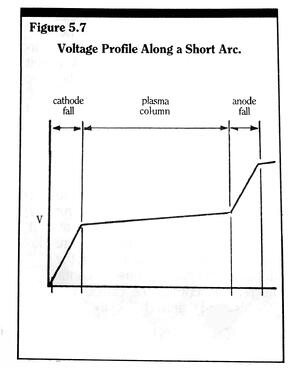
By short, we mean that the voltage drop across the plasma column is small in comparison to the combined voltage drops across the cathode and anode fall regions.  Typically, this will occur when the physical length of the plasma column is small.  The cathode and anode fall regions are the transition regions between the metallic cathode and anode electrodes and the gaseous plasma column.  The magnitudes of the electric fields within the cathode and the anode fall regions are much higher than the magnitudes of the fields within the metallic cathode and anode.  And, much higher than the magnitude of the field within the plasma region.  Higher electric fields are, by definition,  higher voltage drops per unit distance, and thus the use of the term “fall,” as in “voltage fall” in the descriptions of the cathode and anode transition regions.

The voltage drops or “falls” within the cathode and anode fall regions are strong functions of the materials used as cathode and anode electrodes, but relatively weak functions of the current level within the arc.  The energy required to completely remove an electron from the surface of a material body is defined as the “work function” of that material.  Expressed as an equivalent voltage (energy divided by the charge of one electron), the vacuum work functions of most metallic elements are approximately 4 to 5 volts.  The detailed physics of electron emission and collection in cathode and anode regions under arc conditions is of such complexity that only a limited number of low current, simplified cases have been theoretically analyzed by researchers.  For our purposes, it is sufficient to say that the cathode and anode voltage drops are “of the order” of the cathode and anode work functions.

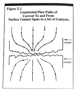
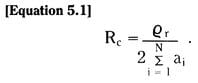
The actual surface area of the cathode electron emission and anode electron collection varies with the total arc current.  The current densities within these active areas, however, are extremely large, particularly so for the cathode.  Current densities exceeding 10⁶ A/cm², and surface temperatures exceeding 4000^oK have been postulated by Lee for cathode “spots”.  At these current densities and temperature electron emission is a combination of thermionic and field emission.  Electrons with enough thermal energy can thermionically escape the surface of the cathode but, due to the large concentration of positive ions in front of the cathode, a high surface electric field is also present.   It enables surface electrons to tunnel through a reduced surface work function energy barrier, and be accelerated away or “emitted” by field emission. 

Even higher surface “spot” temperatures can be present at the anode.  When electrons leave the cathode, they take energy with them.  Therefore, the cathode is actually cooled by their exit (On a net basis, however, the cathode is heated by the I²R heating within the cathode spot and the energy of incoming positive ions).  When electrons arrive at the anode, they dump their energy into the anode surface and heat it up (in addition to the anode I²R heating).

Dependent on the actual surface spot temperatures, anode and cathode evaporated surface material will transfer from hotter to cooler surfaces if the gap is sufficiently small (as in a breaker at initial contact parting).  Some investigators have shown that material transfer can be a function of peak arc current, where the peak surface temperature transfers from cathode to anode as the peak arc current increases beyond a certain threshold.

The plasma column in an arc is composed of a partially ionized gas.  Gas molecules are “ionized” when neutral gas molecules separate into negatively charged free electrons and positively charged ions.  This occurs by a number of different processes:  high electric field electron and positive-ion collisions; absorption of radiation; and thermal ionization, ionization by means of collisions with high temperature (i.e. high energy) electrons, positive ions and neutral molecules.  All of these processes occur in an arc; the relative importance of each is dependent on location within the plasma column and the strength of the arc.  The energy input to the plasma column is the Joule heating due to mobile current carriers.

Since there is a large difference between the mass of an electron and the mass of a positive ion, there is a large difference between the response of an electron and a positive ion to an applied electric field.  By far, the majority of the current within the plasma column of an arc is carried by electrons.  Therefore, the initial energy transfer to the plasma is to the electron gas within the plasma.  But very rapidly, by means of collisions, this energy is shared with the plasma positive ions and the background neutral molecules.  Thus, in time intervals of interest to the circuit breaker design engineer, and to a very good degree of approximation, the plasma is in a state of thermal equilibrium.  That is, all components (electrons, ions and neutral molecules) within a spatial region are at the same temperature.

At thermal equilibrium conditions, the rate of ionization within a particular differential region is balanced by an equal rate of ion-electron recombination.  Also, the net concentrations or densities of electrons and positive ions are approximately equal and monotonically dependent on the plasma temperature.

The conductivity of the plasma region in the arc is a strong function of the plasma temperature.  The higher the temperature, the higher the level of thermal ionization and carrier concentration.  The more carriers, the less the value of electric field needed to support a given level of current density (i.e. the conductivity increases).  This positive feedback effect – more current → higher heating → more carriers → more current for a given level of external excitation – partially accounts for the steady-state negative differential resistance of an arc.

Another contributor to the steady-state negative differential resistance of an arc is the cross-sectional spreading of the plasma column at higher current levels.  As the temperature of the active (ionized) plasma column increases, so too does the temperature of the gas surrounding the plasma column due to thermal conduction (and perhaps convection and radiation).  At high enough temperatures above a threshold temperature, the immediate surrounding gas will also undergo thermal ionization.  There will then be additional carriers present to carry the arc current, increasing further the net arc conductivity.

A typical static or steady-state voltage current characteristic of an arc is given in Figure 5.8.

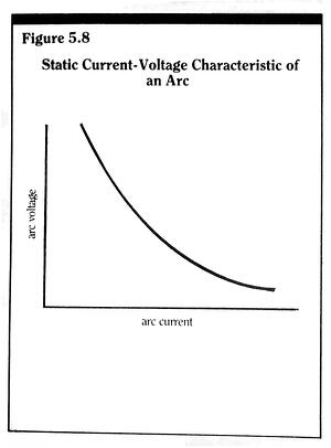
In general, for a given level of arc current, the arc voltage is proportional to the arc length.  But for a given arc length, higher arc currents result in lower arc voltage drops due to the static negative differential resistance characteristic.

A common arc control scheme used in many circuit breaker designs, (i.e. a method used to increase the total arc voltage across the main contacts), is to force the arc into an arc baffle or splitter structure.  A typical arc baffle structure in a small circuit breaker is shown in Figure 5.9.

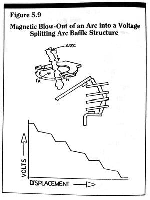
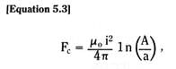
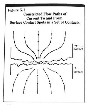
Arc baffles act to break a single arc into several shorter arcs connected in series.  The anode and cathode voltage drops of these multiple arcs then add and comprise a major portion of the total device – arc voltage.  The movement of the arc into the baffle is initiated by the magnetic Lorentz force, or J x B force, due to the arc current itself (J is the arc current density and B is the magnetic flux density due to the current).  This magnetic Lorentz force is the same force which tends to repel the contact faces apart due to constriction current flow paths to minute contact points.  The movement of the arc, due to this self magnetic force, is referred to as magnetic blow-out of the arc.

Magnetic blow-out is also used to force arc movement onto arc “runners”, which are attached to the contact structures (see Figure 5.10).

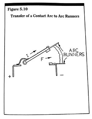
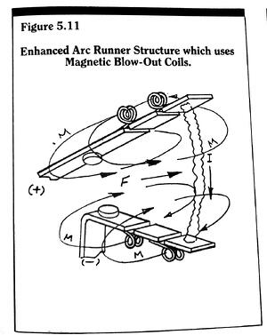
Use of arc runners preserves the more expensive silver alloy contact material by moving the cathode/anode “feet” of the arc off the contacts, and onto the less expensive runner material.  In addition, the arc runners present a longer arc path for the arc to traverse, and can act as the transfer medium between the inter-contact region and any arc baffle or arc chamber region.  Arc runners can be enhanced with the addition of staged electromagnetic drive coils to even further strengthen the magnetic blow-out force along the runner length. (see Figure 5.11).

In circuit breaker design and analysis the static characteristics of the arc are certainly of interest, but, it is the dynamic characteristics of the arc that are of prime concern.  The arc carries the circuit current until an interruption will be successful, that is, whether or not the arc will reignite as the voltage across the breaker contacts rises, is a question that can only be answered by a study of the arc dynamic behavior.

In a typical circuit breaker, upon release of the restraining latch the movable-contact arm will begin to accelerate.  The dynamic behavior of the movable arm is determined by the effective mass of the arm, the strength and preloading of the drive spring, the magnitude of the current through the contacts, frictional forces on the arm hinge and arm travel, and the speed and detailed action of the latch release mechanism.

Since the current flow is constricted and forced to flow in converging paths to contact spots on both bulk contact faces, as shown in Figure 5.1, there will be components of current flow which are anti-parallel to each other within the adjoining contacts. 

These anti-parallel components form single-turn “loop” inductors.  These inductors tend to expand in an effort to minimize their self-inductance, and thus minimize their stored magnetic energy.  The magnetic force which acts to expand the current loop inductors is then a net repulsion force between the two bulk contacts.  Holm [5.1], Snowdon [5.2] and a number of others,

have shown that the repulsion force due to the current constriction in a single contact spot is approximately given by

where i is the magnitude of the instantaneous current through the contact spot, a is the effective radius of the single contact spot, and A is the effective radius of the total bulk contact surface area.  This force of electromagnetic repulsion adds to any mechanical forces which tend to separate the contacts.  By itself, it is generally small in comparison to the movable contact spring force, except under high current conditions.  At high currents the repulsion force (due to the current squared term in Equation 5.3) can become significant, even dominant, in certain structures [5.3].

This repulsion force has even been utilized in the construction of a mechanical AC fault current limiter [5.3].  In this device, movable contact arms, are restrained together by a spring mechanism (see Figure 5.2a).

Under very high fault current levels the electromagnetic repulsion between the contact arms overcomes the restraining springs and forces the contacts apart.  Figure 5.2b illustrates that the resulting arcis longer than that needed in a normal AC breaker.  It thus has a very high arc voltage, which “bucks” the fault current drive voltage, and limits the peak fault current to values less than that which would flow without the arc voltage in series with the faulted circuit.

The mechanical dynamics of the parting of circuit breaker contacts are very similar to the dynamics of the armature of a magnetic circuit breaker.  Barkan [Equations 5.4, 5.5 and 5.6] has presented detailed studies of contact dynamics for large, electric utility type breakers.  The theory of small light duty breakers, however, is very similar. 

Figure 5.3 shows a simplified contact mechanism.

This figure is an adaptation of Barkan’s Figure 2 given in reference [5.4].  Barkan obtained closed form solutions for the system shown in Figure 5.3 for the following situations:  (a) ideal system, lumped concentrated masses, no drag forces, negligible electromagnetic force, and instantaneous latch release;  (b) as in (a) but with a finite latch release time;  (c) as in (a) but with viscous drag proportional to the square of the moving contact velocity; (d) as in (a) but with distributed but rigid contact linkages; and (e) as in (a) but with distributed flexible contact linkages.  We will restrict our interest to only cases (a) and (b).

For an ideal system, case (a), we have for the equation of motion for the movable contact

where m is the equivalent mass of the movable contact (including the contact arm), x is the contact position measured from complete contact closure, k is the drive spring constant, and x_s is an equivalent position which is proportional to the initial force on the contact immediately after latch release.  If the latch releases instantaneously at time = 0, we have for the solutions of (5.4)

where ω is the angular velocity  v(t) is the contact velocity, x_o is the initial contact position ( = 0 at start) and v_o is the initial contact velocity ( = 0 at start).

If the latch does not release the contact instantaneously then the initial forcing term in (5.4) must be modified.  From strain gauge measurements during latch release Barkan [5.4] found that a latch restraining force drops off approximately as a cubic time function.  Thus, the equation of motion becomes

where T is the time required for the latch to completely release the contact arm.  The solutions to (5.7), valid for 0<t<T and zero initial position and velocity are given by

and

For t > T we can use (5.6) and (5.7), with initial conditions given by (5.8) and (5.9) evaluated at t=T, and with time t given by t—T.

We plot the contact position x, normalized to the equivalent initial force position X_s, for both instantaneous and non-instantaneous latch release in Figure5.4.

In this plot we have assumed that the non-instantaneous release is completed in two tenths of the spring-mass cycle time, that is, ωT/2π = 0.2.  The corresponding contact velocity plots for these cases normalized to ωx_s, are given in Figure 5.5 the movable contact “average” velocity v_av

Also normalized to ωx_s.  Typical measured values for average velocities for small circuit breaker structures are 20-300 cm/sec.

If the movable contact is not on a spring loaded arm, but rather on a flexible snapaction bi-metal structure, the simple equation of motion, Equation 5.4, does not apply.  The actual dynamics of a snapping structure are quite complex, but the end result, a co-sinusoidal (in time) like movement is quite similar to that of a simple spring loaded arm.

Figure 5.6 is a plot of the measured displacement of a contact on a snap-action low power toggle switch [5.7].  The solid line is the measured result taken from a high speed film.  The dashed line is an empirical fit of the data to an equation of the form

Where x_ss is the steady state separation (1.1mm), α= 208 sec^-1, n = 1.45 and ω is the radian mechanical frequency.  For this structure the average velocity at x =͂ 1.0 mm is seen to be

The device current in thermal and magnetic circuit breakers passes through both a detection mechanism and a set (or sets) of electrical contacts.  The contacts are generally spring loaded and latch restrained.  When triggered by the overcurrent detection mechanism, the latch will release a movable contact arm.  The arm then withdraws from the fixed contact at a rate determined by spring loading and electromagnetic forces due to the contact current.

When the contacts are closed, or “latched”, current flows between the contacts only at very small physical contact points, or asperities, due to surface roughness on the bulk contact faces.  The actual area of electrical contact is only a small fraction, less than 1%, of the apparent area of the bulk contact surface (see Figure 5.1).

Current flowing in the contact bulk regions is constricted at these contact points, much like fluid flowing through a pipe with an insert containing very small holes.  The extra electrical resistance due to this current restriction is referred to as the spreading or constrictive resistance of the contact.  It can be shown [5.1] that the constriction resistance on each side of an individual contact “spot” is given by

where ϱ_r is the bulk resistivity of the contact material, and a is the effective radius of the asperity or actual contact spot area.  If the contacts are constructed of two different materials, with respective bulk resistivities  ϱ_r1 and ϱ_r2, the total series spreading resistance due to current constriction in both contacts is

Normally, contacts are fabricated with identical materials and, normally, actual contact is made at N number of spots on the contact surfaces.  The net constriction resistance for the contacts is then the parallel combination of all the individual contact values, or

The effective radius of each contact spot, a_i, is dependent on the preparation of the bulk contact surface, the normal forces applied to the contacts, the “hardness” of the contact material (i.e will each contact asperity be under elastic or plastic deformation?), and the temperature at the contact interface.

In addition to constrictive resistance at contact asperities, there may be a resistance due to a thin film or layer of material oxide between contacting asperities.  Electrons either tunnel quantum mechanically through this thin film, or break through the film by a process Holm refers to as “fritting” [5.1].  The film resistance is between the constriction resistances of individual asperities, so the net “contact” resistance would be a modification of Equation (5.1):

where R_fi is the film resistance at asperity i.

In practice there is no attempt to determine contributions to R_contact due to individual contact spots.  The net excess resistance of the contact system, beyond the bulk resistances of the two contacting bodies, is simply referred to as the contact resistance.  The voltage drop across this resistance is commonly referred to as the contact drop.  In most cases this contact drop does not exceed .1-.2 volts.  Contact drops tend to saturate at these levels since, as the magnitude of the current rises, the asperity interface temperature rises softening the asperity material.  The softer material spreads out and increases the actual asperity contact area, thus lowering the contact resistance.

When two bulk metallic contacts which are carrying an electrical current separate, the last point or points of physical and electrical contact will be at one or more (if more than one, a small number) constriction asperity spots.  The current density at these points will be very large, easily enough to melt the asperity material and form molten bridges between the two contacts.  These bridges are then heated and stretched to the point that they vaporize.  The process initiates the arc between the two contacts.  If the contacts are not metallic, such as carbon, the asperity points do not melt, but rather arc immediately upon physical separation.  

In comparison, to the detection time response of thermal circuit breakers, we can classify the detection time response of magnetic circuit breakers as “fast”.  In many cases, magnetic breakers are in fact “too fast”, and are subject to nuisance trips due to transient inrush currents.  Whereas thermal breakers can “ride through” transient inrush currents by means of their relatively long thermal time constants, magnetic breakers tend to respond to the instantaneous magnitudes of inrush currents due to their relatively low trip energy requirements once the threshold current has been exceeded.

Over the years magnetic circuit breaker designers have developed several schemes to delay the detection response to transient inrush currents.  In essence, the goal is to mimic the dual element “slow blow” fuse structure.  The ideal “dual element” magnetic breaker would have two detection mechanisms in series:  one slow, low threshold current mechanism to ride through inrush currents; and one fast, high threshold current mechanism to quickly respond to true, high level fault currents.  The detection time current response characteristic would look much like the dual-element fuse characteristic shown in Figure 3.9.

A true, almost ideal dual-element characteristic can be achieved in a magnetic circuit breaker through use of an inertial core-delay tube.  This clever device is shown in Figure 4.13a.  The drive coil core is a hollow tube which contains a moveable, but spring restrained core ferromagnetic slug.  At low coil currents the slug is spring restrained in a recessed position, x = 0.

At coil currents above a certain operating current threshold, I_th1, the attractive magnetic force (solenoid effect) of the coil is enough to overcome the spring force and to initiate movement of the slug.  The slug moves toward the coil center and begins to fill the hollow coil core with ferromagnetic material.  As the coil core fills with magnetic material the core section reluctance falls to lower values, enabling the total magnetic flux produced by the coil to increase.  When the core slug reaches a certain point in the core section, dependent on the level of drive coil current, the core reluctance is decreased to a value low enough that the magnitude of the armature gap flux is sufficient to cause the armature to breakaway from its stopped position.  The breaker then trips as described previously.

The dynamics of the slug movement can be further slowed by the addition of a viscous fluid within the hollow core section.

If the initial core current is high enough – above a second threshold level I_th2 – the gap flux will be strong enough to trip the armature without the need of flux enhancement by slug movement through the core section.  The dynamics of this high-level trip are then the fast dynamics of a pure, simple magnetic breaker, unaffected by the flow dynamics of the core slug mechanism.

In terms of a magnetic equivalent circuit, the moveable-core dual element magnetic circuit breaker can be described as shown in Figure 4.13b.  The core path reluctance R_c is now a function of the slug displacement from its restrained x = 0 position.  It is a maximum when the slug is at x = 0, and a minimum when the slug has advanced to its core-filled position at x = x_max.

The equation of motion for the slug is given by

where M_s is the mass of the core slug, F_m is the force of the magnetic attraction on the slug, D is the coefficient of friction due to the addition of a viscous fluid environment, ξ is the spring constant of the slug restraint spring, and x_o is an equivalent displacement representing the initial restraining force of the spring.  The force of magnetic attraction F_m will be proportional to the core flux ф squared (just as the armature attractive torque T_m is proportional to the gap flux ф_g squared).  A complete solution to the dynamics of the total device would then require a simultaneous solution of Equations 4.1 and 4.18, and the magnetic circuit of Figure 4.13b.

We will not attempt to solve this system of equations here.  We will only note that the “slow” behavior of the complete system is determined by the slug movement Equation 4.18; the “fast” behavior of the system is determined by the armature movement of Equation 4.1; and coupling between the two is determined by the magnetic circuit, Figure 4.13b.  The resultant combined detection time-device current characteristics are sketched in Figure 4.13c.

Other methods of desensitizing the response of magnetic breakers to inrush currents include the tailoring of the core flux reluctance path as a function of the core slug position and the addition of an inertial device, similar to a flywheel, to the armature structure.

Flux can be “bled-off” from the core-gap-armature path through use of flux shunts (sometimes referred to as flux busters) or through the use of an elongated core path which is not covered by the drive coil.  In either situation a major portion of the core flux produced by the drive coil tends not to flow  through the core-armature gap until a movable internal core slug (similar to the one in Figure 4.13a) has reached its fully advanced position.  Rather, this flux “bleeds” into leakage paths, producing no useful armature torque.  However, when the core slug is at its most advanced position these leakage paths are effectively “shorted” and the major portion of the core flux crosses the core armature gap.  Magnetic breakers with these tailored core flux paths have an enhanced, true, dual-element response characteristic.

Extra inertial mass when added to the armature mechanism increases the total effective armature moment of inertia, or equivalently, the total effective armature characteristic time.  This addition does not change the sensitivity of the detection mechanism; it only slows its response.  It slows it, however, across the board.  It does not create the desired dual-element response; rather it simply burdens the armature with additional inertia, enabling it to ride through the transient inrush currents by means of sheer sluggishness.

The production of magnetic flux is instantaneously proportional to the coil current i.  Strictly speaking, this is only true for magnetic circuits which do not contain any electrically conductive magnetic flux paths.  When the level of magnetic flux changes (i.e. is raised or lowered) in a path/medium which can also conduct electric current, such as iron, there will arise, by Faraday’s Law, circulating eddy currents.

(Faraday’s Law states that the voltage induced in any closed path in space is proportional to the time rate of change of the net magnetic flux which flows through the closed path cross-sectional area.  If the closed path is in an electrically conducting medium, there will then be a circulating current around that closed path proportional to the generated voltage and the electrical conductivity of the medium).

These eddy currents will, in turn, produce reaction magnetic flux which will tend to cancel out a portion of, or all of, the original excitation flux.  The direction of eddy current flow can be deduced by the “ right hand rule” and by the requirement that the reaction magnetic flux produced by the eddy currents must flow in the opposite direction to the flow of excitation flux.  Eddy current production in a simple cylindrical path in iron is illustrated in Figure 4.11.

As a result of eddy currents, flux cannot be instantaneously produced in conducting mediums.  There will always be a time “lag” between the flux flow and the exciting mmf.  A simple magnetic equivalent circuit representation of this time-delay effect can be made by including “inductive” elements in series with reluctance elements which represent electrically conductive paths.  For example, the structure shown in Figure 4.4 has two magnetic paths which are made up of ferromagnetic material: the core path and the armature path.

We include eddy current effects in these two paths by placing inductive elements in series with the reluctive elements which represent these paths.  This modified circuit is shown in Figure 4.12.

The value of the inductive element for each magnetic path in a conducting medium is a function of the cross-sectional geometry of the path, the electrical conductivity of the material, and the effective length of the path.  In the simple cylindrical structure of Figure 4.11, it can be easily shown that the equivalent eddy current inductance L_e is given by

where L is the axial length of the conductor and ϱ_r is the electrical resistivity of the material.  The magnetic reluctance of this path is

where µ_m is the magnetic permeability of the material , A is the cross-sectional area = πr², and r is the cylinder radius.  The magnetic time constant τ_e of this cylindrical path is then

As typical values, let the material be a 1.5mm radius rod of magnetic iron with µ_m=˜ 2000µ_o and ϱ_r = 10^-5Ω-cm.  Thus,

If such a rod is used as a magnetic core in a magnetic circuit breaker, and if we wish to accurately predict the breaker time response over time intervals of this magnitude, we must then necessarily include eddy current effects in our calculations.  We can no longer use the simple results for the gap flux calculated from the static circuit of Figure 4.4.  Rather, we must use the dynamic circuit of Figure 4.12.  Results such as those given in Figures 4.9 and 4.10, calculated using static equivalent magnetic circuits, are optimistic at predicted operating time intervals equal to or less than the eddy current time constants of the structure elements.

For a rectangular cross-section magnetic path with side length ratio k, the equivalent eddy current inductance can be shown to be equal to

The path lengths of eddy currents in a rectangular cross-section magnetic conductor are longer than those in circular cross-section magnetic conductor.  Thus, for equal electrical conductivities, the effective eddy current inductance in a rectangular conductor is lower.

To mitigate eddy current effects in magnetic materials, we see from Equations 4.16 and 4.17, that we should construct magnetic cores with

1)     Magnetic irons (steels) with high resistivity values, (i.e. silicon steels). And

2)     Very thin sheets (i.e. laminations) of magnetic steels stacked in the thin direction, and oriented such that the thin direction is perpendicular to the flow of magnetic flux.

The cost of such construction is only justified for devices which must operate at very high speeds (i.e. operating periods of the order of milliseconds).

We can recast the equation of motion.

Equation 4.1, in dimensionless form by dividing through by the breakaway torque T_B.  We obtain

The quantity J_aθ_g/T_B has units of (time)², so we define a characteristic time t_a for a magnetic breaker as

This “time” is seen to be a function of the inertia of the armature, the spring constant of the armature restraining spring, the amount of pre-load we place on the restraining spring, and the angular width of the armature air gap.  Each different magnetic breaker will have its own particular value of t_a.  But in terms of t_a, all magnetic breakers of similar design will have the same dynamic behavior.

If we assume the idealized case of no latch mechanism load torque (i.e. T_latch = 0), we will not need to consider impact effects when the armature slams into the latch mechanism.  This case will also be the minimum time response, or fastest possible response, for a magnetic structure.  The normalized equation of motion can then be written as

We can easily solve this differential equation numerically for any given set of values for the frame reluctance fraction m, normalized coil current i/I_th, and gap angle – spring pre-load angle ratio θ_g/θ_o.  Example solutions for m = 0.1, θ_g/θ_o  = 1.0, and different values of step input i/I_th are given in Figure 4.9.

The latch mechanism trips the contact separation mechanism when the armature angle reaches the latch threshold value θ_th.  The time required to trip the contact separation mechanism, measured from the overcurrent inception, is the detection time of the breaker t_d.  We plot the detection time response for the example solutions given in Figure 4.9 as a function of input normalized overload current in Figure 4.10.

In this case we have assumed that the threshold armature angle is 80% of the armature gap angle.  As can be seen, the normalized detection time is a monotonically decreasing function of the normalized input current.

In the case of no armature saturation, at high values of input current (in the example of Figure 4.10 for i>5I_th), the detection time becomes linearly dependent on the ratio I_th/i.  This linear behavior at high input currents can be deduced directly from the normalized equation of motion.  At high input currents the armature angular acceleration is approximately proportional to (i/I_th)² only.  Thus a simple double integration gives

From which we see that

for a given threshold angle θ_th.

If armature saturation occurs, the time response of the armature will be slowed slightly.  The detection times for a saturated case would be slightly higher than non-saturated values, such as those given by the solid line in Figure 4.10.Saturated values would tend to level off at a minimum detection time since the drive torque would also saturate at a maximum value, given by (4.9) using the saturated gap flux value.  A typical saturation case is shown by the dashed line response in Figure 4.10.

Magnetic circuit breakers have DC threshold currents.  When magnetic devices are operated at their threshold levels, the trip or detection times are also “long” times.  Action on the onset of mechanical movement in a magnetic circuit breaker, however, is more abrupt than in a thermal circuit breaker.

Mechanical movement of the thermal element is evident up to the detection threshold value in a thermal breaker.  In a magnetic breaker, there is the possibility of no mechanical action, (i.e. no movement whatsoever) until the threshold current is exceeded.

From the equation of motion (4.1) we have that there will be a net accelerating torque on the armature at angular position θ = 0 whenever

where we have assumed that the latch mechanism is not engaged until θ>˭θ_latch.  We will term the torque value ƴθ₀, the breakaway torque T_B.  If we now plot the load torque – the restraining spring plus latch mechanism – as a function of armature angular position, we obtain a load torque locus such as that shown in Figure 4.5.

Note that we have approximated the load torque of the latch as a constant average torque, <T_latch>, over the operating range of latch mechanism.  We also show the load torque diminishing (dashed line) after the latch release angle θ_th.  In truth, we care little as to the actual behavior of armature after tripping, and therefore the true locus after this point is of no concern.

From Equations 4.9 and 4.11,

we see that the driving torque of magnetic attraction T_m is given by

The current needed to produce a torque of magnetic attraction equal to the breakaway torque will be termed the threshold current I_th, and is defined by the expression

Equation 4.12, the equation for the magnetic torque, can then finally be written in a compact form as

We can now plot, for a given value of frame reluctance fraction m and various values of constant coil current i, the value of magnetic drive torque T_m as a function of the armature angle θ.  These curves are shown, along with the load torque curve T_L, in Figure 4.6.

The difference between the drive torque T_m and the Load torque T_L at any value of armature angle θ, is the acceleration torque.  Once the threshold current I_th has been exceeded, the net acceleration torque T_m – T_L is seen to increase as the armature approaches its closed position.  This is a positive feedback effect, contributing to the “fast” characteristic behavior of magnetic circuit breakers.

In some magnetic breakers, the positive feedback effect is diminished somewhat by magnetic saturation of the armature iron.  As the armature gets closer to its closed position, the gap reluctance becomes smaller.  Thus, the total reluctance of the armature-gap path also becomes smaller, which for constant coil current, induces higher levels of armature-gap flux.  If this level of flux approaches the saturation level of the armature, the effective armature reluctance R_ca begins to rise, and thus the frame reluctance fraction m begins to rise as well.

The effect of a rising value of m, due to armature saturation for a constant coil current i, is shown in Figure 4.7. 

Here, curves of drive torque T_m at constant coil current i, but varying values of frame reluctance fraction m, are plotted as functions of the armature angle θ.  If armature saturation occurs as θ approaches θ_g, the actual trajectory of T_m would be along a curve, such as the one shown as T_m (sat).  The net accelerating torque over the operating range of θ is thus seen to diminish, if armature saturation is present.

We have defined the threshold current as that coil current which induces a value of magnetic torque of attraction equal to the armature breakaway torque.  There are situations, however, where this definition is inadequate.  For example consider the drive torque – load torque case shown in Figure 4.8.

Here, an impressed coil current is of sufficient magnitude such that

                                              T_m (θ = 0) > T_L (θ = 0)

so the armature would start to move.  But, at an armature angle value θ_A, less than the latch angle θ_th, the drive torque curve crosses over the load torque curve.  This cross over point, point A, is a stable operating point (net accelerating torque for θ<θ_A and net decelerating torque for θ>θ_A), and thus motion will stop at A.  The “trip” threshold drive torque curve for this situation is shown by the dashed line in Figure 4.8.

Situations such as the one shown in Figure 4.8 should be avoided in the design of magnetic circuit breakers.  Breakers designed as in Figure 4.8 will always exhibit a certain value of armature overshoot, beyond angle θ_A, due to the armature inertia.  If this overshoot is large enough, the latch mechanism could be tripped inadvertently.  Rather than depend on the uncertain impact behavior between an overshooting armature and the latch mechanism, the design of a magnetic circuit breaker trip-threshold should be based on the behavior indicated in Figure 4.6.  Namely, no armature movement should occur until the coil current exceeds the threshold value.  We can insure this type of response simply by requiring that the drive torque curve never cross-over the load torque curve at any value of θ, including θ>θ_latch.

The magnetic flux ф_g that flows through the air gap in the structure of Figure 4.2, is a portion of the total flux generated by the current flowing in the coil which surrounds the core material. 

This total flux ф, which flows through the coil enclosed cross sectional area, is produced by the coil current and is proportional to both the magnitude of the coil current i and the total number of turns N of wire that makes up the coil.  The product of N and i is referred to as the magnetomotive force, or mmf, of the coil.  The proportionality factor in the relationship between the total flux produced by the coil current and the coil mmf, has units of flux (measured in webers) per unit mmf (measured in ampere-turns). 

Since the total flux ф is proportional to a force term – the mmf – a simple analogy can be made between a magnetic circuit and an electrical circuit.  In a DC electrical circuit the current i flows due to an electromotive force (emf) E.  Ohm’s Law for an electrical circuit states that

where R is the resistance of the circuit to the flow of current.  A “Magnetic Ohm’s Law” is then

where R is the resistance of the magnetic circuit to the flow of flux.  This resistance to flux flow R has been assigned a special name to differentiate it from resistance to current flow.  We refer to it as the reluctance of the magnetic circuit.

The reluctance of a magnetic circuit will be approximately constant as long as the flux density in any one portion of the circuit is below the saturation flux density for that portion of the circuit.  Ferromagnetic materials become saturated with magnetic flux at density levels of approximately 1-2 Teslas = 1-2 webers/(meter)².  At density levels near this saturation value, the effective reluctance of the material rises rapidly.  At density levels below the saturation value, the reluctance of ferromagnetic elements is far below that of comparable sized elements constructed of non-magnetic materials.

To construct a representation of a simple lumped magnetic circuit for the magnetic circuit breaker structure of Figure 4.2, we must remember that the total flux created by the coil to be made up of two components:  a gap component ф_g which flows through the coil, the core structure, the armature and the gap, and a leakage component ф_ᵜ which flows through the coil, a portion of the core structure and a leakage air path.  Figure 4.4a illustrates the two components flowing in their physical paths.

Figure 4.4b illustrates an electrical equivalent “magnetic circuit” for the device.  Here, the coil mmf is shown as a DC voltage source of magnitude Ni, and the magnetic reluctances of the different flux paths are shown as equivalent resistances.

The reluctance portion of the core which carries both the leakage flux and the gap flux is labeled R_c;  the reluctance of the air path portion of the leakage flux path is labeled R_ᵜ; the reluctance of the core and armature portion of the gap flux path is labeled R_ca;  and the gap reluctance is termed R_g.  The actual values of the reluctances R_c, R_ᵜ, R_ca and R_g are determined by the effective cross sectional areas of the respective flux paths, the effective lengths of the respective flux paths, and the magnetic permeabilities of the respective flux paths.  If the path material is a ferromagnetic material, such as iron, the path reluctance will also be a function of the level of flux density within the path, if the density level is near or above the saturation value.

In general, for any given path, we have for the path reluctance

where L_p is the effective length of the path, A_p is the effective cross sectional area of the path, and µ_p is the magnetic permeability of path medium.  If the path medium is ferromagnetic, at high levels of path flux, ф_p, flow, we have µ_p = µ_p (ф_p).  Since the gap flux and the leakage flux are both air paths, both path permeabilities equal the permeability of free space µ_o – which is a strict constant, and not a function of path flux level.

For the gap we have approximately

where θ_g is the angular opening of the gap measured with the armature at its held position.  If we define

we then have

Now from simple DC circuit analysis of the circuit of Figure 4.4b, we have

or, if we normalize the circuit reluctance as “seen” from the gap, R_ca  + R_ᵜ  R_c /(R_ᵜ + R_c)to the maximum gap reluctance R_gmax, and let this ratio be termed the frame reluctance fraction m, we have

Since the core and armature are constructed with magnetic materials, we have in general,

This last result suggests that the frame reluctance fraction m is a small quantity.  At high levels of core or armature saturation, however, these approximations become less accurate and the value of m will grow.  Some devices are constructed with a “time-engineered” value of R_c.  For the “time-engineered” devices, the core flux path reluctance R_c is high for a portion of their operating time.  Thus the above approximations are also invalid.

It is well known that electromagnets can exert a lifting or attractive force on ferromagnetic materials, such as iron.  The force mechanism is the same mechanism by which permanent magnets attract iron objects.  Simply stated, near the surfaces of a magnetic material (a ferromagnetic material, one which has a low resistance to the flow of magnetic flux), the density of the energy stored in the magnetic field is much higher on the exterior than on the interior of the material.  By the principal of virtual displacement, there will be a mechanical pressure in the direction of the outward normal at the surface of the magnetic material.  Since there will be more magnetic field flux at the surfaces of the material that are closest to a nearby magnet, or electro-magnet, the total net force on the magnetic material body will be an attractive force, towards the magnet or electromagnet.

Consider the electromagnet structure shown in figure 4.1

In it a coil of N turns of wire is wrapped around one leg of a ferromagnetic core structure.  A movable ferromagnetic armature is hinged to another leg of the core structure.  At one end position of swing the armature closes the core structure and completes a closed path of ferromagnetic matter through which magnetic flux can flow.  The armature is held away from the core closing position by a spring mechanism, creating a classic "relay" structure.

Coil current will induce magnetic flux within the core material, the armature material, and in the gap between the armature and the coil leg of the core.  At a sufficient level of coil current the magnetic attractive force on the armature will exceed the retention force of the spring and the armature will move to its core closed position.  If, by its movement, the armature can trip a latch mechanism - releasing a spring driven contact opening mechanism - then based on the level of coil current, we have a trip/no trip decision mechanism (i.e. we have a magnetic circuit breaker).

A simplified armature-latch release mechanism is shown in Figure 4.2.

Observe that the armature's path is composed of two sections, a free-movement (spring constraint only) portion, and a latch release (spring constraint and latch restraint force) portion.  It is similar to the deflection path of the bi-metallic element in a creep type thermal circuit breaker.

 The equation of angular motion of the armature (see Figure 4.3) is given by

where θ is the armature’s angle, measured from its completely restrained position; θ_o is an angle measure of the initial pre-load on the restraining spring; γ is the torsional spring constant of the restraining spring; T_latch is the torque load of the latch release mechanism (T_latch = 0 during the free movement portion of the armature travel); T_m is the torque due to magnetic attraction, and J_a is the effective angular moment of inertia for the entire armature structure.

In equation 4.1 we have neglected all friction effects due to the armature hinge and air movement.  For this structure, the detection time t_d is defined as the time, measured from the overcurrent inception, required for the armature angle θ to advance to the point of latch release.  We will define this latch release angle as θ_th.

Before discussing the dynamic behavior of the armature, that is, solutions to (4.1), we will first examine the nature of the magnetic torque T_m.  Neglecting any magnetic flux paths through the top surface of the armature structure, the total magnetic torque on the armature is given by

where the surface integral is taken over the entire armature bottom surface (the surface on the core side), p_m is the magnetic pressure on the armature bottom surface, and r is the moment arm of the differential force p_m dA.  Since the armature is made of iron, the direction of magnetic flux flow through its exterior surface will be almost perfectly normal to the surface.  In this case, the magnetic pressure [4.1] is given by

where B_n is the magnitude of the normally directed magnetic flux density vector at the armature surface, and µ_o is the magnetic permeability of free space (µ_o = 4π x 10^-7 henries/meter).  The magnetic permeability of a medium is a measure of the medium’s ability to conduct the flow of magnetic flux.  Magnetic materials have relative permeabilities several thousand times that of free space.  The total net magnetic force F_m on the armature, directed towards the core structure, is given by

And the total magnetic flux ф_g, which flows through the bottom surface of the armature, and therefore, through the gap between the armature and the core, is given by We can now define an effective gap cross-sectional area A_g by equating the two force expressions

Such that

This effective gap cross-sectional area allows us to think of the armature as a free body, with a uniform magnetic pressure F_m/A_g, acting on a portion (A_g) of its lower surface.  We can even define an effective moment arm r_q for a point force F_m by equating

So that

If the distribution of normal magnetic flux over the bottom surface of the armature does not change as the armature position or the driving coil current changes, the effective cross-sectional area of the gap A_g, and the effective armature moment arm r_q, will both be constant (See Equations 4.6 and 4.8).The total magnetic torque on the armature is now simply given by

Equation 4.9 indicates that in order to increase the magnetic torque for any given armature structure, we need only increase the total gap flux.  And, for a given input current, we need only to control the time development of the total gap flux, if we wish to control the time response of a magnetic breaker detection mechanism.

In a bi-metal thermal circuit breaker, the elements expand in longitudinal directions, but the major or useful mechanical movement is in a lateral direction to the elements.

 Consider the two blade elements, 1 and 2 shown in Figure 3.15a.

A blade is a body with an elongated, rectangular cross-section, and with overall length L much greater than either the width b or thickness h.  Both blades have equal length L_o at a reference temperature T_o.  But, at temperature rise ΔT = T-T_o, blade 2 is longer than blade 1, L₂>L₁, because the difference in the two coefficients of thermal expansion, α_t2>α_t1.

If we now bond the two blades together while at the reference temperature, to form a single blade of thickness h = h₁ + h₂, we produce a bi-metal blade element see Figure 3.15b).  Now, at temperature rise ΔT, blade 2 will try to expand to length L₂, but will be “held back” by its bond to blade 1.  Blade 1 wants to expand only to length L₁, but it is “pulled” to a length greater than L₁ by its bond to blade 2.  Thus, blade 2 is subjected to an overall longitudinal compressive force P₂, while blade 1 is subjected to an overall tensile force P₁.  Since there is no movement of the total free body when the elevated temperature is held constant, these two forces must be equal and opposite along the length of the total composite blade.  The curvature seen in Figure 3.15b, will be concave (an inside curve) on the blade 1 side and convex (an outside curve) on the blade 2 side.

The formal definition of concave curvature is

We might (correctly) suspect that for small values the concave curvature of the composite blade would be proportional both to the temperature rise ΔT of the blade and to the difference in coefficients of thermal expansion of the two blade materials.  That is,

and K is a proportionality constant which would be a function of the elasticity of each blade material and the thickness of each blade.  Neglecting small end effects, the radius of curvature should be a constant along the length of the composite blade, so that K should not be a function of the original length L_o.  K should also not be a function of the width b, if L_o is several times larger than b, since the major bending will only be along the longitudinal axis.

The original derivation of the proportionality constant K is credited to Villarceau, who published his work in Paris in 1863.  The standard English language derivation of K is the classic 1925 paper of Steven Timoshenko, “Analysis of Bi-Metal Thermostats.”  In this paper Timoshenko not only derived the bending constant K, he also presented for the first time, the theory of “snap action” thermostat behavior. 

Timoshenko has shown that for an amazingly large range in elastic material constants, and for an amazingly large range in blade thicknesses, the bending constant K can be approximated as

Figure 3.16 illustrates that for a free blade, we can them solve for the maximum mid-blade deflection ό as follows:

The curved blade arc angle φ is given by

where ΔL is the composite blade terminal expansion.  But for small deflections, L_o/r is already small so that the term ΔL/r is of second order and can be neglected, thus, φ =~L_o/r.

The cosine of φ/2, by the construction shown in Figure 3.16, is

which for small φ can be approximated by

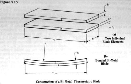
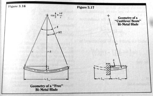
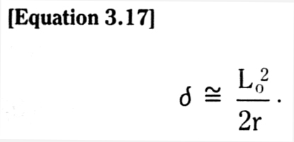
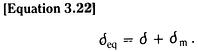
For a blade built into a fixed wall – a cantilever beam – we see from Figure 3.17 that the blade end deflection is exactly the same as the mid-blade deflection of a free blade of initial length 2L_o.  Thus, for a cantilever blade of initial length L_o, we have for the blade end deflection

Note that for equal lengths, the maximum deflection of a cantilever blade is four times that of the free blade.  We can now combine (3.14) and (3.15) with deflection Equations 3.16 and 3.17 to obtain:

Normally a creep bi-metal blade must not simply deflect - it must also exert a force on a latch release mechanism during a portion of, or during all of, its deflection trajectory. 

From the elementary theory of uniform beam deflections, we have for the configurations of Figure 3.18 that the deflections for a concentrated mechanical force P_m are

where E is the effective Young’s modulus of elasticity for the composite blade.  It follows that a bi-metal blade will exert a concentrated force P_m if it is constrained such that if it was free it would deflect by an amount ό_m.  Thus, to calculate the temperature rise ΔT needed to deflect a blade by an actual distance ό, and to exert force P_m, we use the equivalent deflection ό_eq,

This equivalent deflection would be used in place of the actual deflection ό in Equations 3.18 and 3.19.

Let us subtract from any free deflection ό_f that a blade would travel before exerting any mechanical force on a latch mechanism.  This free travel deflection would be subtracted from the total actual deflection ό, and the total equivalent deflection ό_eq.  We then have

where we can define

an equivalent free deflection while exerting a mechanical force on the latch mechanism and

an actual deflection while exerting a mechanical force on the latch mechanism.  So that

If we assume that the average amount of work, W_m, expended in tripping the latch mechanism is equal to a constant average mechanical force P_m, times the action distance ό’, using (3.18) through (3.21) for both free and cantilever blades, we have

where we differentiate between free and cantilever blades by the factor β, where

and ΔT’ is the temperature rise needed to deflect the blade a total equivalent distance of ό’_eq.  We can simplify (3.24) and place it in the form

where the constant W_k = 9/64 β⁴E (Δα_t)², m = ό_m/ό’_eq and L_obh is the total volume of the blade material.  Thus, for a given latch mechanism which requires energy W_m to trip, and for a given desired operating temperature rise ΔT’, we can determine the most economical blade design - (i.e. the minimum volume design) if we minimize the expression for the total blade volume

with respect to the normalized suppressed mechanical travel m = ό_m/ό’_eq.  By taking the derivative of (3.25) with respect to m, and setting it to equal zero, we find that the optimum design is one with

That is, the suppressed deflection should be equal to the actual deflection when the blade is in the process of exerting a mechanical force.  Any other choice of deflection ratios will result in an increase in the required volume of bi-metallic material, and thus an increase in material cost.  Note that the amount of free travel that the blade undergoes before it begins any mechanical work has no effect on the optimum choice of suppressed blade deflection.  This free travel only influences the total amount of temperature rise that is needed to complete the total equivalent deflection.

As a practical example of a minimum volume design, consider the use of Chace No.2400 bi-metal material in a cantilever blade latch release mechanism.

In our notation, the manufacturer supplied data for this representative material is given in Table 3.1.  Assume that the blade must, after some length of free deflection, push against a latch mechanism with an average force of one once.  And to trip the mechanism the blade must travel 0.05 in. while applying this force.  The work required to trip the latch is then

Further assume that we wish this work to be accomplished by a deflection due to temperature rise ΔT’ = 50^oF.  From Equation 3.25 with W_k = 5.74 x 10^-3 1bf/(in^2oF), the minimum volume of material that is capable of performing this work (i.e. the m = ½ design), is given by

A commonly available thickness value for bi-metal material is 0.008 inches.  If we choose this value for h, and assume an active blade length of ¾ inch, we see that we need a blade width of,

Note that this minimum volume design satisfies our original assumptions of a “blade” device, one with a length several times greater than width or thickness.

The time it takes for a creep bi-metal element to trip a latch release mechanism is the time it takes to heat the element to the required total temperature rise ΔT = ΔT_f,+ΔT’, where ΔT_f, is the temperature rise during any free deflection of the element before it begins any latch release work.  We can safely neglect any inertial effects due to the bi-metal element itself.  The stiffness of bi-metal material insures that the transient or natural mechanical response of the element is completely negligible in comparison to the driven mechanical response for any reasonable level of heat application.  This can be easily seen if one calculates the period of the fundamental frequency of natural vibration of a bi-metal element.  This period is much less than the time needed to raise the temperature of the element to the value dictated by the required total deflection.  Thus the time-current detection period characteristics of a directly heated bi-metal element can be determined exactly like those of a hot-wire element.  That is, we can use Equation 3.9, with suitable values for the constants: threshold current I_th, element resistance temperature sensitivity factor k, and element thermal time constant Ƭ. 

For an indirectly heated bi-metal element, the thermal equivalent circuit is more complicated than the simple two element model.  An indirectly heated element analysis must, at a minimum, involve two thermal time constants – one for the actual heating mechanism and one for the bi-metal element itself.

For a directly heated element we can solve for the time-current response using Equation 3.9 as follows:

1)      1) Choose a desired threshold temperature rise ΔT = ΔT_f + ΔT’.

2)      2) For the particular blade element material, find the resistance temperature factor k from

3)      3) Integrate (3.9) numerically.

As an example, let us solve (3.9) for Chace No. 2400 material.  If we choose a threshold total temperature rise of 200^oF, we have

The actual value of the long time threshold current I_th is best determined experimentally since it depends on the thermal resistance R_t, which is unknown and not easily theoretically determined.  In normalized form, the solution for stepped DC currents for the detection time t_d, the time required to reach T_th, is given in Figure 3.19.

In general, due to the differences in thermal capacity, the thermal time constants for hot wire breakers will be smaller than those of thermal creep-blade breakers.  Thus, the actual detection times, for equal ratios of operating current to threshold current, will be related by

T_d (hot wire)< t_d (creep-blade)

Finally we note that thermal “creep” type breakers must be derated at high ambient temperatures.  However, by special design, such as the addition of a second bi-metal (complimentary) mechanism, thermal breakers can be ambient temperature compensated.  These compensated mechanisms show little variation over their specified operating temperature range.